Data Engineering · DuckDB · ETL
Fetching Airport Weather Data in Brazil with DuckDB
Using DuckDB, CLI to perform a quick ETL and spatial visualization
Fetching Airport Weather Data in Brazil with DuckDB
The goal is to perfom a simple ETL and combine with geospatial information for quick visualization.
DuckDB Env setting
First, we install all the extensions:
INSTALL h3 FROM community;
INSTALL lindel FROM community;
INSTALL json;
INSTALL parquet;
INSTALL spatial;
Then we create a .duckdbrc, which is a configuration file. It loads whenever we run a query.
touch .duckdbrc
nano .duckdbrc
Then paste
bash
.timer on
.width 180
LOAD h3;
LOAD lindel;
LOAD json;
LOAD parquet;
LOAD spatial;
Note: since I am running this inside a Docker Compose, I have created this step when mounting the container, so I don’t have to worry about this step.
Filtering Data from Brazil
We have build a asos.sql file where a table is created with readable names and filtered for Brazil only.
CREATE OR REPLACE TABLE weather_br AS
    SELECT {
        altitude: alti,
        elevation: elevation,
        latitude: latitude,
        longitude: longitude,
        country: country,
        county: county,
        name: name,
        state: state,
        station: station
        } AS location,
        {
            tzname: tzname,
            valid: valid
        } AS time_,
        {
            celcius:tmpc
        } AS temperature,
        vsby AS visibility,
        {
            gust:gust,
            direction: drct,
            knots: sknt
        } AS wind,
        {
            celcius:dwpc
        } AS dewpoint,
        {
            one_hour_meters: p01m
        } AS precipitation,
        mslp AS mean_sea_level_pressure,
        relh AS relative_humidity
    FROM 'https://data.source.coop/dynamical/asos-parquet/year=2024/data.parquet'
    WHERE country='BR';
Now, it’s possible to validade whether there is some data or not:
duckdb -json asos.duckdb -c "SELECT * FROM weather_br LIMIT 5;"
Bingo!
{
"location":
    "{
        'altitude': 30.0,
        'elevation': 34.0,
        'latitude': -22.8751,
        'longitude': -43.3847,
        'country': BR,
        'county': NULL,
        'name': Rio De Janeiro,
        'state': BR,
        'station': SBAF
    }",
"time_":
    "{
        'tzname': America/Sao_Paulo,
        'valid': 2024-01-01 10:00:00+00
    }",
"temperature":
    "{
        'celcius': 24.0
    }",
"visibility":6.21,
"wind":
    "{
        'gust': NULL,
        'direction': 270.0,
        'knots': 1.0
    }",
"dewpoint":
    "{
        'celcius': 14.0
    }",
"precipitation":"
    {
        'one_hour_meters': 0.0
    }",
"mean_sea_level_pressure":null,
"relative_humidity":53.55
},
Counting the amount of airports weather registry in Brazil
- How many registries are there in Brazil?
echo "SELECT count(*) FROM weather_br"   | duckdb  asos.duckdb
# Output: 762609
- How many in 2024?
echo "SELECT count(*) FROM weather_br WHERE time_.valid BETWEEN '2024-01-01'::DATE AND '2024-12-31'::DATE "   | duckdb  asos.duckdb
#Output: 760573
Basically, all records are within the same year.
Verifying the average temperature per day
The query is in the file 01_asos.sql, and for simplicity, it’s filtered for december only. A Parquet file will be generated to save for a later plot.
/*Get the average temperature per day */
COPY(
    SELECT
        time_.valid::DATE AS date_calendar,
        avg(temperature.celcius) AS mean_temperature_c
    FROM weather_br
    GROUP BY 1
    ORDER BY date_calendar DESC
) TO './asos_day_avg_temp.parquet' (FORMAT parquet)
Once the query is set, we can run it in the terminal with:
duckdb asos.duckdb < 01_asos.sql
Result:
|date_calendar  │ mean_temperature_c │
│     date      │       double       │
├───────────────┼────────────────────┤
│ 2024-12-31    │ 25.960700757575758 │
│ 2024-12-30    │ 25.707202993451823 │
│ 2024-12-29    │ 25.665248226950354 │
│ 2024-12-28    │ 26.041958041958043 │
│ 2024-12-27    │ 25.531876138433514 │
│ 2024-12-26    │ 25.204513399153736 │
│ 2024-12-25    │ 25.606017191977077 │
│ 2024-12-24    │ 25.639282341831915 │
│ 2024-12-23    │ 25.554432705558106 │
│ 2024-12-22    │ 25.676128431828758 │
│ 2024-12-21    │   26.1012832263978 │
│ 2024-12-20    │  26.45578231292517 │
│ 2024-12-19    │  26.19972514887769 │
│ 2024-12-18    │ 25.938505203405867 │
│ 2024-12-17    │ 25.892592592592592 │
│ 2024-12-16    │ 26.156411460779708 │
│ 2024-12-15    │  25.51631912964642 │
│ 2024-12-14    │  25.37883797827114 │
│ 2024-12-13    │ 25.756143667296787 │
│ 2024-12-12    │  25.68302945301543 │
│ 2024-12-11    │ 25.382851902796883 │
│ 2024-12-10    │ 25.788251366120218 │
│ 2024-12-09    │ 25.796728971962615 │
│ 2024-12-08    │  25.86112401300511 │
│ 2024-12-07    │  26.60401119402985 │
│ 2024-12-06    │ 26.555864626796478 │
│ 2024-12-05    │ 25.380794701986755 │
│ 2024-12-04    │ 24.709073900841908 │
│ 2024-12-03    │ 25.512968299711815 │
│ 2024-12-02    │ 26.776084949215143 │
│ 2024-12-01    │ 27.034741784037557 |
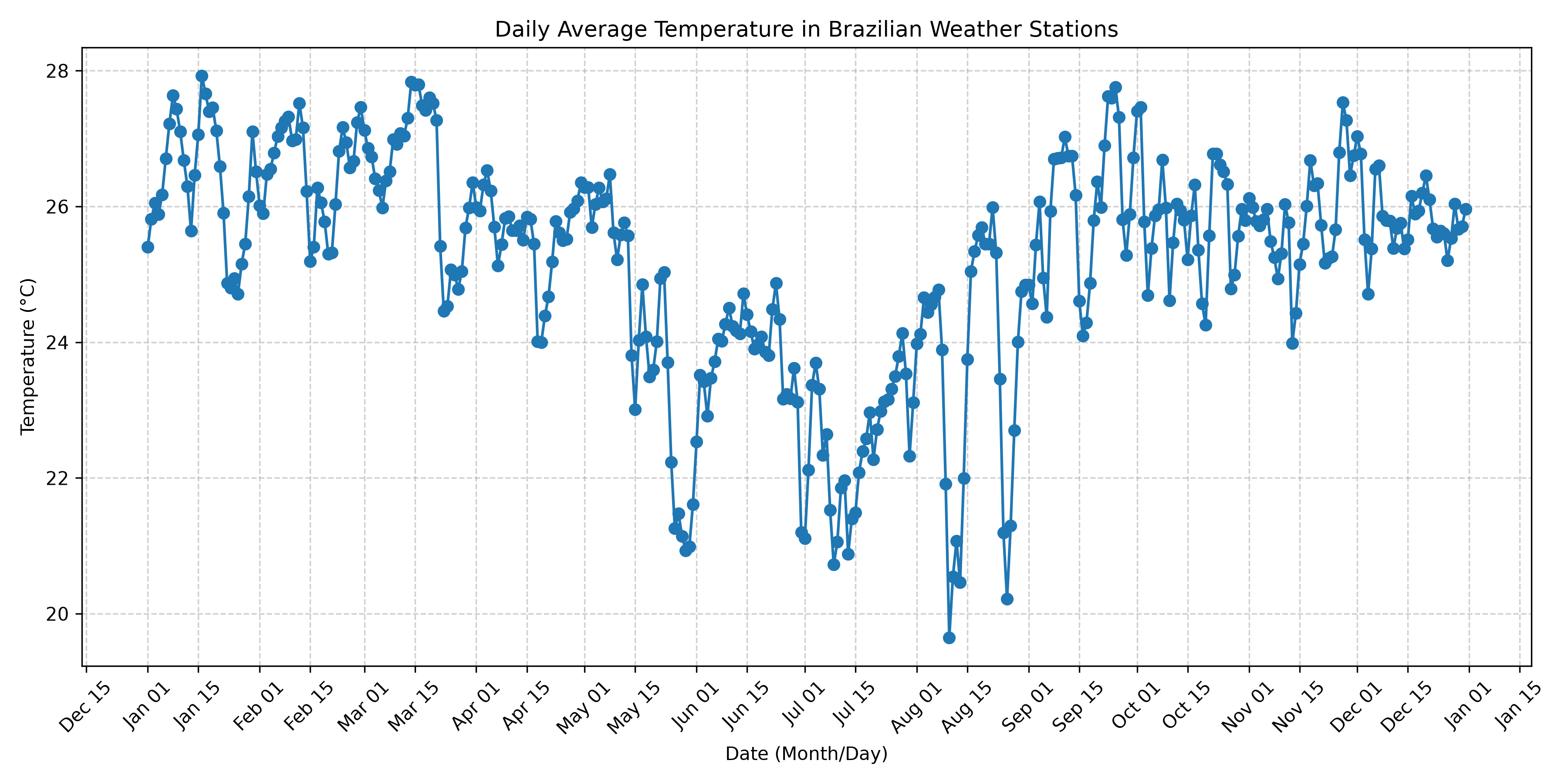
Count by month
In 02_asos.sql I count the occurrences by month and the average temperature.
Let’s check the query first:
/*Get the average temperature per day */
SELECT
    monthname(time_.valid::DATE) AS date_month,
    avg(temperature.celcius) AS mean_temperature_c,
    count(*) AS total_registers
FROM weather_br
GROUP BY 1
ORDER BY 1 ASC
Now, same as before, we run it:
duckdb asos.duckdb < 02_asos.sql
And the result shows that the registers per month is quite consistent, and that Brazil’s average temperature barely changes. Important highlighting that in the sourthern part you’ll have a wider temperature range than in the northern part. When we take the average for the whole country, this temperature range is shrinked, making us interpret that the whole country has mild temperature the whole year long (which is not true!).
┌────────────┬────────────────────┬─────────────────┐
│ date_month │ mean_temperature_c │ total_registers │
│  varchar   │       double       │      int64      │
├────────────┼────────────────────┼─────────────────┤
│ April      │  25.58432281414693 │           62996 │
│ August     │ 23.575232630272954 │           64480 │
│ December   │ 25.842250048855284 │           66523 │
│ February   │  26.53034139237783 │           60429 │
│ January    │ 26.360011915213846 │           63784 │
│ July       │  22.49433821587785 │           64379 │
│ June       │  23.77161952229918 │           61796 │
│ March      │ 26.472156692326795 │           64432 │
│ May        │ 24.234510305659143 │           64091 │
│ November   │ 25.810511493980098 │           63207 │
│ October    │ 25.816488122962273 │           64410 │
│ September  │  25.99595696014948 │           62082 │
├────────────┴────────────────────┴─────────────────┤
Now, let’s see the spatial distribuition of the stations
Simple thing, just add a point geometry and ready to display on QGIS.
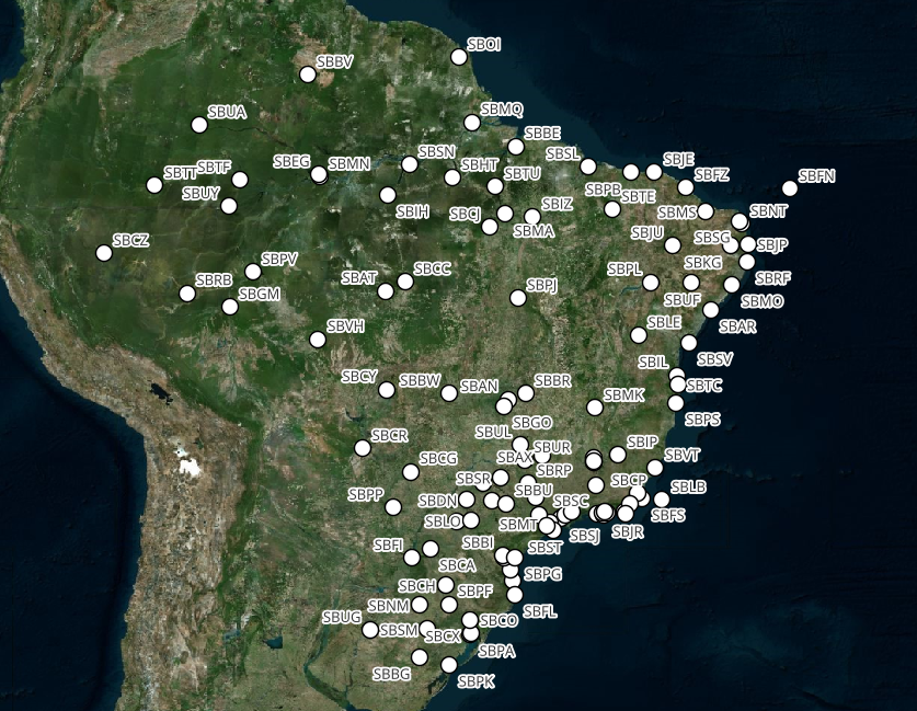
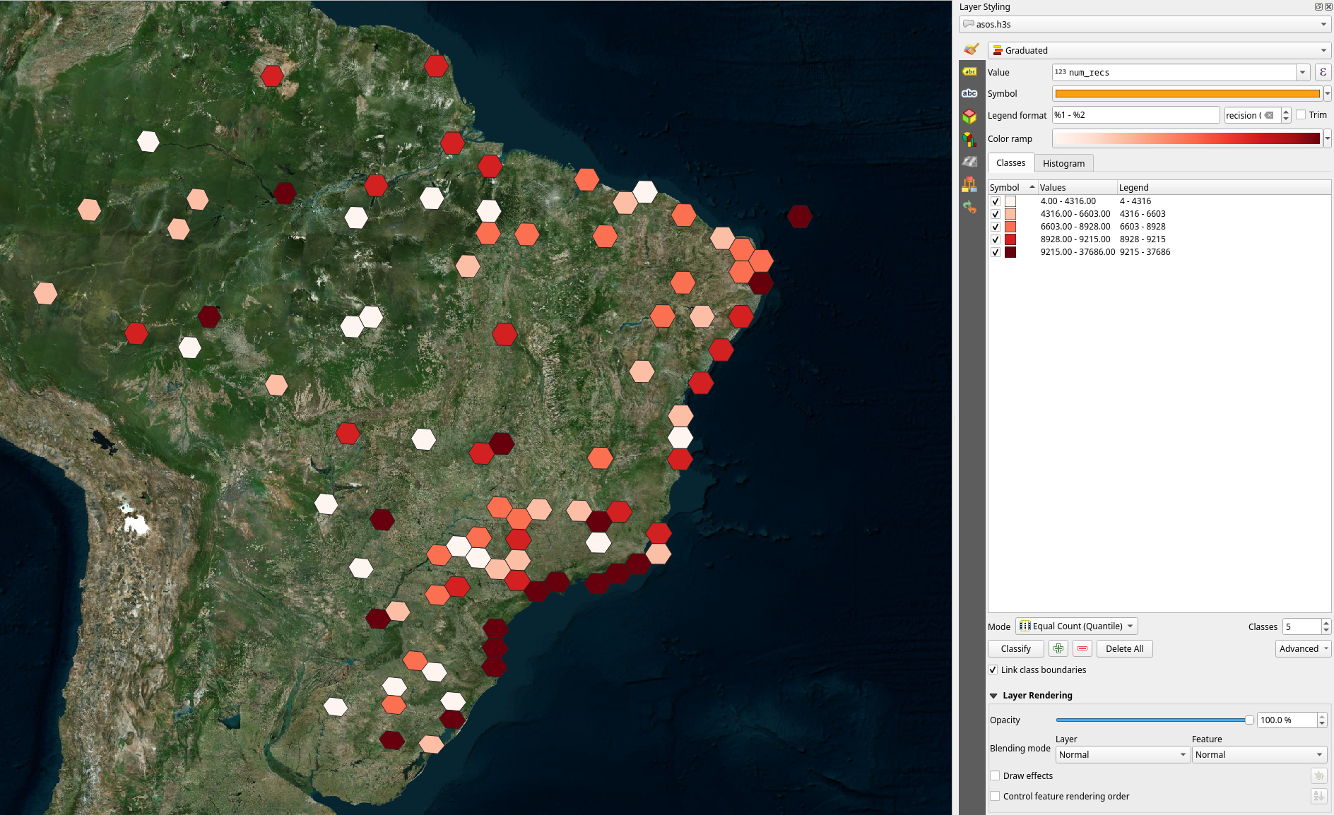
Finally, a concentration map of regions with biggest amount of registers
We can see the amount of temperature registers are around the main cities by the shore, mainly in Sudeste.
Sources & Inspiration
This was written based on Mark Litwintschik’s post. His content has been helping me develop better skills at DuckDB and big data handling.