Satellite Image Classification with OBIA

Introduction

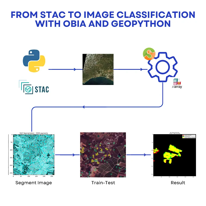
For many daily tasks, using AI makes is look cool, however the problem could be tackled with older techniques, yet with good performance, specially when we take into consideration the cost-benefit ratio: it takes less processing time and does not decrease our metrics sharply.

One of these techniques that can still be used is Object Based Image Analysis (OBIA). AKA GeoOBIA when we apply it on satellite images.

This methodology is usually my first go-to when I need to solve a problem. If its results are already good enough, we don’t need to use a bazooka to kill a couple of ants.

What’s OBIA?

As the name suggests, it deals mainly with objects. With OBIA, when we have an image, we are not analyzing the pixels anymore but groups of pixels with similar characteristics. These grouped pixels are generated by segmentation algorithms, such as SLIC and Quickshift. Of course, you can use newer segmentation algorithms, such as SAM, but it does not necessarily improve the segmentation, and consume more computational resources.

The overall idea is quite simple: identify objects by its color (spectral response) and shape. The workflow consists of three main steps:

1. Segmentation: we group neighboring pixels according to their pixel similarity (shape, color, texture), and then we form polygons, which are the objects.

2. Features Extraction: we calculate the statistical and geometrical characteristics for each object.

3. Classification: after that, we usually apply some classification algorithm, which can be either supervised or unsupervised.

Let’s go through a little project I did in python, using geospatial libraries to classify solar panel farms in Southern Spain. The whole project can be found in my GitHub repository:

1. Image Acquisition

First step is to get the image for the area of interest (AOI). For this task, we are going to use Spatio-temporal Catalog Asset (STAC) specification. It is a quite fast and simple manner of getting up-to-date images without downloading a bunch of images manually.

We select a provider, and then, check all the collections available:

#Set api address and check collections
api_url = 'https://earth-search.aws.element84.com/v1'
client = pystac_client.Client.open(api_url)
for collection in client.get_collections():
    print(collection)

<CollectionClient id=sentinel-2-pre-c1-l2a>
<CollectionClient id=cop-dem-glo-30>
<CollectionClient id=naip>
<CollectionClient id=cop-dem-glo-90>
<CollectionClient id=landsat-c2-l2>
<CollectionClient id=sentinel-2-l2a>
<CollectionClient id=sentinel-2-l1c>
<CollectionClient id=sentinel-2-c1-l2a

The collection of interest is Sentinel-2 Level L2A, so that’s the chosen one.

Following the selection of the collection, we must indicate the AOI, data range, and search the whole catalog to check whether there are images or not.

collection = 'sentinel-2-l2a'

#coordinates AOI
lat = 37.364
lon = -6.923
point = shapely.geometry.Point(lon, lat)
date_range = '2025-04-01/2025-05-16'

search = client.search(
    collections = [collection],
    intersects=point,
    datetime=date_range,
    query = ['eo:cloud_cover<10']
)

items = search.item_collection()
print(f'There are {len(items)} items.') 

# output
There are 2 items.

To better visualize the metadata from images, let’s transform the output into a data frame.

item_df = gpd.GeoDataFrame.from_features(items.to_dict(), crs = 'EPSG:4326')
item_df 

One very important thing is: we don’t want clouds in our image. So, the next step is filtering the images that have cloud percentage below 5%.

ids= item_df.loc[
  (item_df['eo:cloud_cover'] <= 5) &
  (item_df['s2:nodata_pixel_percentage'] <= 4.1)
]

item = items[ids.index[0]]

2. Generating a Data Cube

Since the thumbnail is not useful, it is necessary to transform it to a geoarray, where we can save the metadata and perform analysis. For this step, I like using Xarray.

#generating cube
assets = ["red","green","blue","nir", 'swir16', "scl"]
cube_all = stackstac.stack(
    item, 
    assets, 
    bounds_latlon = bbox, 
    epsg=32629
    )
scl = cube_all.sel(band=["scl"])
s2_mask = da.isin(scl, [3,8,9])
cube = cube_all.where(~s2_mask)
cube = cube.to_dataset(dim = 'band')

#stacking to have RGB composition
rgb = np.dstack((
    normalize(cube['red'][0,:,:]),
    normalize(cube['green'][0,:,:]),
    normalize(cube['blue'][0,:,:])
    )
)
plt.imshow(rgb)
plt.axis('off')
plt.show()

#calculate NDVI
ndvi = ndvi_calc(
    normalize(cube.red), 
    normalize(cube.nir)
    )

plt.imshow(ndvi[0,:, :], cmap = 'RdYlGn', vmin = -1, vmax = 0.95)
plt.colorbar()
plt.axis('off')
plt.show()

I think it would be nice to add it to the cube. I’ll also add other band compositions that I think will be helpful for the classification task

#Adding NDVI to the datacube
cube['ndvi'] = ndvi

#generating agriculture composition
agriculture = np.dstack((
    normalize(cube.swir16[0, ...]),
    normalize(cube.nir[0, ...]),
    normalize(cube.blue[0, ...])
))

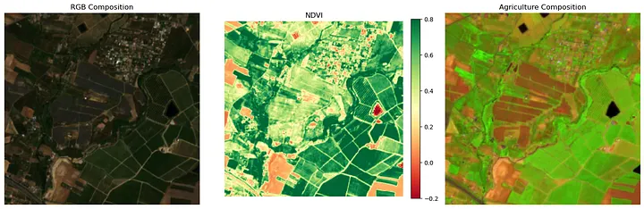
Ok. Now, we have our data cube with a couple of indices. The next step is doing the image segmentation.

3. Image Segmentation

The segmentation will generate polygons with similar characteristics. For that, we use skimage library. The chosen segmentation function was SLIC.

# amount of segments what will be generated
n_segments = 1000
compactness = 8

segments = slic(rgb, n_segments=n_segments, compactness=compactness, start_label=1)

ndvi = cube.ndvi[0,...].to_numpy()

#plotting the NVDI with segments on top
fig, ax = plt.subplots(nrows = 1, ncols=3, figsize = (15,10))

ax[0].imshow(cube.ndvi[0,...], cmap="RdYlGn", vmin = -0.2, vmax = 0.8)
ax[0].set_title('NDVI Image')

ax[1].imshow(label2rgb(segments, ndvi, kind='avg'), cmap="RdYlGn")
ax[1].set_title('Average NDVI for cell')

ax[2].imshow(mark_boundaries(
    ndvi, segments, color = (0,1,1), mode = "thick"
    ), vmin = -0.2, 
    vmax = 0.8, 
    cmap = 'RdYlGn'
)
ax[2].set_title(f"SLIC Segmentation - {n_segments} segments")

plt.tight_layout()
plt.show()
n_segments = 1000
compactness = 8

segments = slic(rgb, n_segments=n_segments, compactness=compactness, start_label=1)

Now, with our custom function to calculate characteristics for each segment.

Now that the objects were generated, and now they have spectral characteristics, we can perform the train and test, one step closer to our classified image.

Train and Test

Now, a couple of segments will be manually classified, so later a Random Forest can be trained.

To make things simple, we are doing a binary classification. Basically, select what is a solar panel (yellow) and what is not (green).

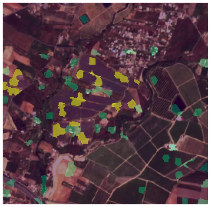
The next step is to split the data and run the RF model.

#Start training
labeled_segments = all_feats[all_feats['class'] != -1]

X_train = labeled_segments.drop(columns = ['label','class'])
y_train = labeled_segments['class']

clf = RandomForestClassifier(n_estimators=100, random_state=42, oob_score=True)
clf.fit(X_train,y_train)

print('OOB Score:', clf.oob_score_)
OOB Score: 0.9428571428571428

Finally, we run the model in the whole image again so we can have our classification map:

mapped_rf_classification= map_array(
    segments,
    np.array(all_feats["label"]),
    np.array(all_feats["class"]))

fig, axs = plt.subplots(ncols=2, figsize=(15, 10), constrained_layout=True)

# Display the original RGB image
axs[0].imshow(rgb_stretch)
axs[0].set_title("Original RGB")

# Display the prediction result
axs[1].imshow(mapped_rf_classification, interpolation="nearest")
axs[1].set_title("Random Forest classifier prediction")

# Remove axis for all subplots
for ax in axs:
    ax.set_axis_off()

# Display the combined figure
plt.tight_layout()
plt.show()

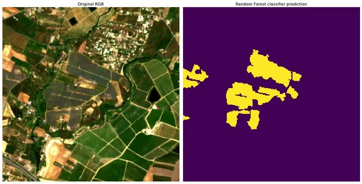
To perform the evaluation of the classification, we used OSM dataset for the region. Basically, we queried the solar panels that felt within the AOI.

The selected metric was Intersection over Union (IOU), to measure the overlap between a predicted bounding box and a ground truth bounding box.

With very little code, processing power and in a quick prototyping, the result was around 84.4%.

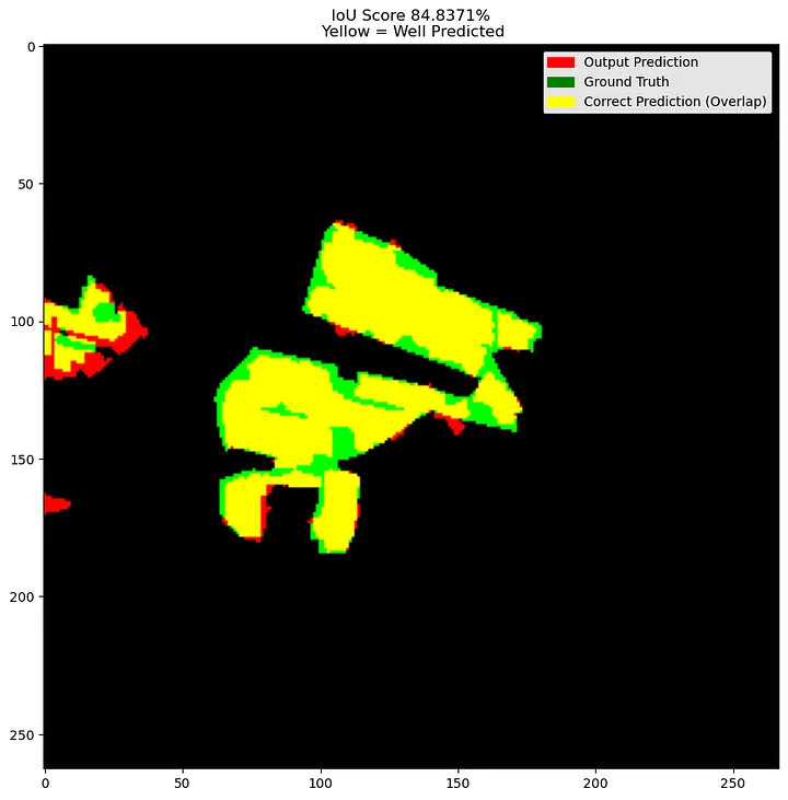
This shows how we can achieve good results without needing to waste computational power. The result could be improved by increasing the amount of features for the model to learn better, or even doing a better feature analysis to identify the relevant ones.

That’s why I argue that many times we don’t need to use heavy AI on our imagery. We already have very good methods that can be used and are quickly to deploy.